Tier 1 Sea Ice Changes CMIP6 f_out 3.2%
CMIP6 Envelope Comparison
DestinE anomalies compared to the CMIP6 P5–P95 percentile envelope derived from 37 ensemble members across 8 models under SSP3-7.0.
Contributing models: CNRM-CM6-1, EC-Earth3, MIROC6, MPI-ESM1-2-LR
Outside CMIP6 does not mean wrong — it indicates an uncommon response within the CMIP6 distribution.
Synthesis
Related diagnostics
Sea Ice Concentration Change (NH)
| Variables | avg_siconc |
|---|---|
| Models | ifs-fesom, ifs-nemo, CMIP6-MMM |
| Units | 0-1 |
| Baseline | 1990-2014 |
| Future | 2040-2049 |
| Method | Future mean minus historical mean. |
Summary high
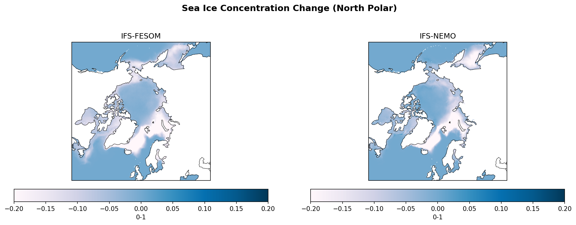
This figure illustrates annual sea ice concentration changes (2040-2049 vs 1990-2014) in the Arctic. Both high-resolution IFS models project strong sea ice declines primarily in the marginal ice zones (Barents, Kara, and Greenland Seas), whereas the CMIP6 multi-model mean predicts a much more extensive loss penetrating deep into the Central Arctic basin.
Key Findings
- All models consistently show a reduction in sea ice concentration across the Arctic, with no regions of significant increase.
- IFS-FESOM and IFS-NEMO exhibit very similar spatial patterns, confining the strongest losses (> 0.2 fraction) to the Marginal Ice Zones: Barents Sea, Kara Sea, Greenland Sea, Baffin Bay, and Hudson Bay.
- The CMIP6-MMM shows a markedly different pattern in the Central Arctic, with widespread deep declines (> 0.15 fraction) across the pole, where the IFS models show negligible change (white/pale pink).
- Both IFS models preserve a 'stable' central ice pack (in terms of concentration) for this period, unlike the CMIP6 average.
Spatial Patterns
The IFS models display a 'ring-like' structure of sea ice loss along the continental shelves and Atlantic sector boundaries, leaving the central basin relatively intact. In contrast, the CMIP6-MMM displays a basin-wide decline, suggesting a transition towards ice-free summers or significantly reduced annual cover across the entire Arctic Ocean.
Model Agreement
There is strong agreement on the location of retreat in the Atlantic sector (Barents/Greenland Seas) and Hudson Bay. The primary disagreement is the magnitude of loss in the Central Arctic, where IFS models are much more conservative than the CMIP6 mean.
Physical Interpretation
The confinement of loss to the margins in IFS models suggests that ocean heat transport (Atlantic Water inflow) and edge erosion are the dominant drivers of loss in these simulations, or that the baseline central ice pack is sufficiently thick to resist concentration drops by 2040. The widespread CMIP6 loss suggests either thinner baseline ice or stronger thermodynamic melting (albedo feedback) in the coarser models. The high resolution of IFS likely resolves the sharp gradients of the Marginal Ice Zone and ocean eddies better, potentially maintaining a clearer separation between open ocean and the central pack.
Caveats
- Analysis is based on concentration only; sea ice thickness would be required to determine if the central pack is thinning despite maintained concentration.
- The 2040-2049 window captures a transient state; differences may reflect a delay in melting rather than a permanent equilibrium difference.
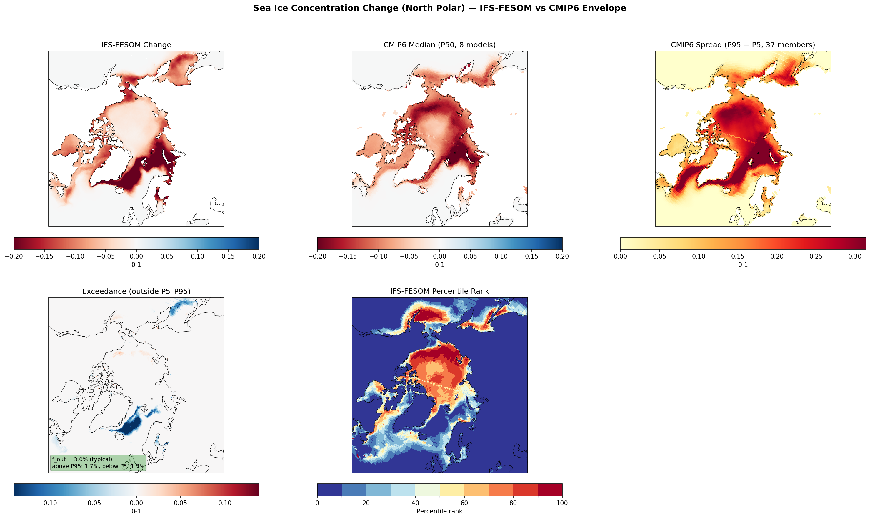
Sea Ice Concentration Change (North Polar) — IFS-FESOM vs CMIP6 Envelope f_out 3.0%
Envelope Metrics
| f_out (outside P5–P95) | 3.0% typical |
|---|---|
| Above P95 | 1.7% |
| Below P5 | 1.3% |
| CMIP6 ensemble | 8 models, 37 members |
| Variables | avg_siconc |
|---|---|
| Models | ifs-fesom |
| Units | 0-1 |
| Baseline | 1990-2014 |
| Future | 2040-2049 |
| Method | Future mean minus historical mean compared to CMIP6 percentile envelope (P5, P50, P95). |
Summary high
IFS-FESOM projects widespread Arctic sea ice concentration loss by 2040–2049, closely tracking the CMIP6 ensemble distribution with a very low fraction of outlier points (f_out = 3.0%). The model exhibits a spatial dipole relative to the ensemble: stronger-than-average sea ice retreat in the Barents Sea sector but weaker-than-average loss in the central Arctic basin.
Key Findings
- Overall agreement with CMIP6 is high; f_out is 3.0%, well within the 'typical' range (<5%), indicating the model behaves consistently with the broad ensemble.
- IFS-FESOM falls below the CMIP6 P5 threshold (blue exceedance) in the Barents Sea and Atlantic inflow region, indicating significantly stronger sea ice loss than 95% of the CMIP6 models in this specific sector.
- In the central Arctic basin, IFS-FESOM ranks in the upper percentiles (60–90th), indicating it projects less intense sea ice concentration decline compared to the CMIP6 median.
Spatial Patterns
The model shows reductions in sea ice concentration (SIC) exceeding 20% across most of the Arctic Ocean. The strongest deviations from the CMIP6 envelope occur at the Atlantic ice edge (Barents Sea), where IFS-FESOM shows 'blue' exceedance (stronger loss), and in the central basin, where high percentile ranks (red/orange) indicate the model retains more ice concentration than the ensemble median.
Model Agreement
Agreement is strong overall. Disagreement is localized: IFS-FESOM is more aggressive in melting the marginal ice zone in the Atlantic sector (Barents Sea) than the CMIP6 envelope, likely due to resolution-dependent differences in ocean heat transport. Conversely, it is more conservative in the deep central basin.
Physical Interpretation
The 'blue' exceedance in the Barents Sea likely reflects the high-resolution FESOM grid's ability to resolve Atlantic Water pathways (Atlantification) more effectively than coarse CMIP6 models, driving stronger basal melt and retreat in that sector. The retention of central Arctic ice (relative to the median) suggests either thicker initial ice or different dynamical export/ice-albedo feedback sensitivities in the high Arctic compared to the CMIP6 mean.
Caveats
- Analysis is based on concentration change only; thickness changes might show different patterns.
- The 3.0% f_out is statistically expected (5% is the definition of the envelope bounds), suggesting the model is effectively indistinguishable from the CMIP6 family globally, despite local differences.
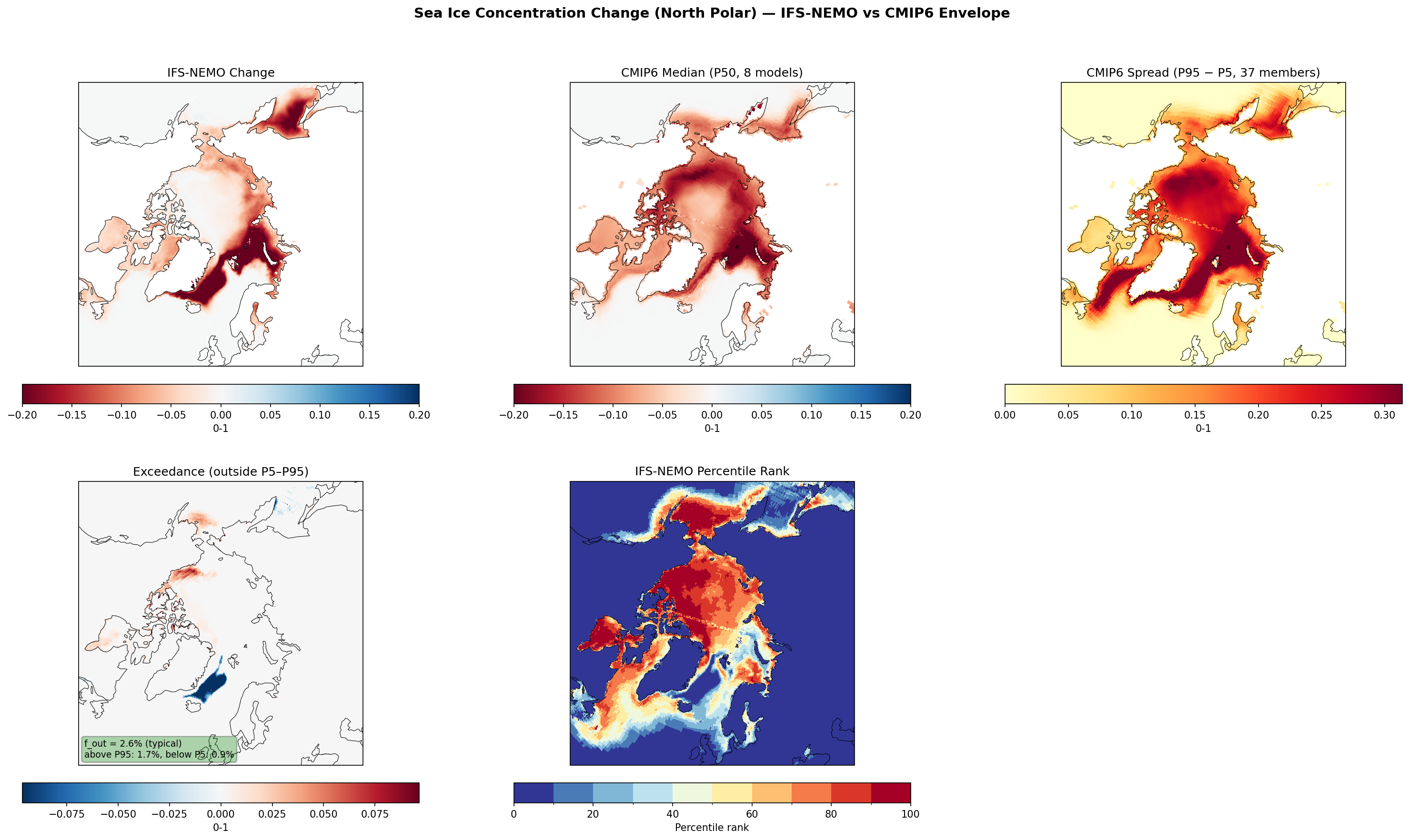
Sea Ice Concentration Change (North Polar) — IFS-NEMO vs CMIP6 Envelope f_out 2.6%
Envelope Metrics
| f_out (outside P5–P95) | 2.6% typical |
|---|---|
| Above P95 | 1.7% |
| Below P5 | 0.9% |
| CMIP6 ensemble | 8 models, 37 members |
| Variables | avg_siconc |
|---|---|
| Models | ifs-nemo |
| Units | 0-1 |
| Baseline | 1990-2014 |
| Future | 2040-2049 |
| Method | Future mean minus historical mean compared to CMIP6 percentile envelope (P5, P50, P95). |
Summary high
IFS-NEMO projects annual sea ice concentration declines for the 2040–2049 period that are remarkably consistent with the CMIP6 ensemble (f_out = 2.6%), with major retreats focused on the Arctic shelves.
Key Findings
- The model shows high fidelity to the CMIP6 distribution, with only 2.6% of the domain falling outside the P5–P95 envelope (classified as 'typical').
- Strongest sea ice loss occurs in the Barents, Kara, and Laptev Seas, closely tracking the CMIP6 median spatial pattern.
- A localized area in the southern Barents Sea shows stronger ice loss than the CMIP6 envelope (blue exceedance), while areas north of Svalbard show slightly weaker loss (red exceedance).
Spatial Patterns
The primary signal is a extensive reduction in sea ice concentration (> -0.15) along the Eurasian shelf (Barents to East Siberian Seas) and in Hudson Bay. The Central Arctic basin remains largely stable in the annual mean, indicating persistent year-round cover or saturation. The CMIP6 spread is widest in these marginal ice zones, reflecting inter-model uncertainty in the exact location of the retreating ice edge.
Model Agreement
Agreement is exceptionally high. The IFS-NEMO percentile rank is close to 50 (median) for most of the Siberian shelf. The main discrepancy is a dipole in the Atlantic sector: IFS-NEMO is in the lower percentiles (stronger loss) in the southern Barents Sea and upper percentiles (weaker loss) north of Svalbard, suggesting a sharper meridional gradient or ice edge than the smoothed CMIP6 ensemble.
Physical Interpretation
The stronger loss in the Barents Sea inflow region likely reflects the high-resolution ocean model (NEMO) resolving vigorous Atlantic Water inflow ('Atlantification') more effectively than coarser CMIP6 models. Conversely, the 'weaker loss' signal in the Canadian Archipelago likely stems from the model's ability to resolve narrow straits and channels that are treated as land or non-dynamic in lower-resolution grids.
Caveats
- Annual means obscure the strong seasonality of sea ice processes (summer melt vs. winter maximum).
- Internal variability in the 2040s (a transition period) can significantly affect decadal means in the highly variable marginal ice zone.
Sea Ice Concentration Change (SH)
| Variables | avg_siconc |
|---|---|
| Models | ifs-fesom, ifs-nemo, CMIP6-MMM |
| Units | 0-1 |
| Baseline | 1990-2014 |
| Future | 2040-2049 |
| Method | Future mean minus historical mean. |
Summary high
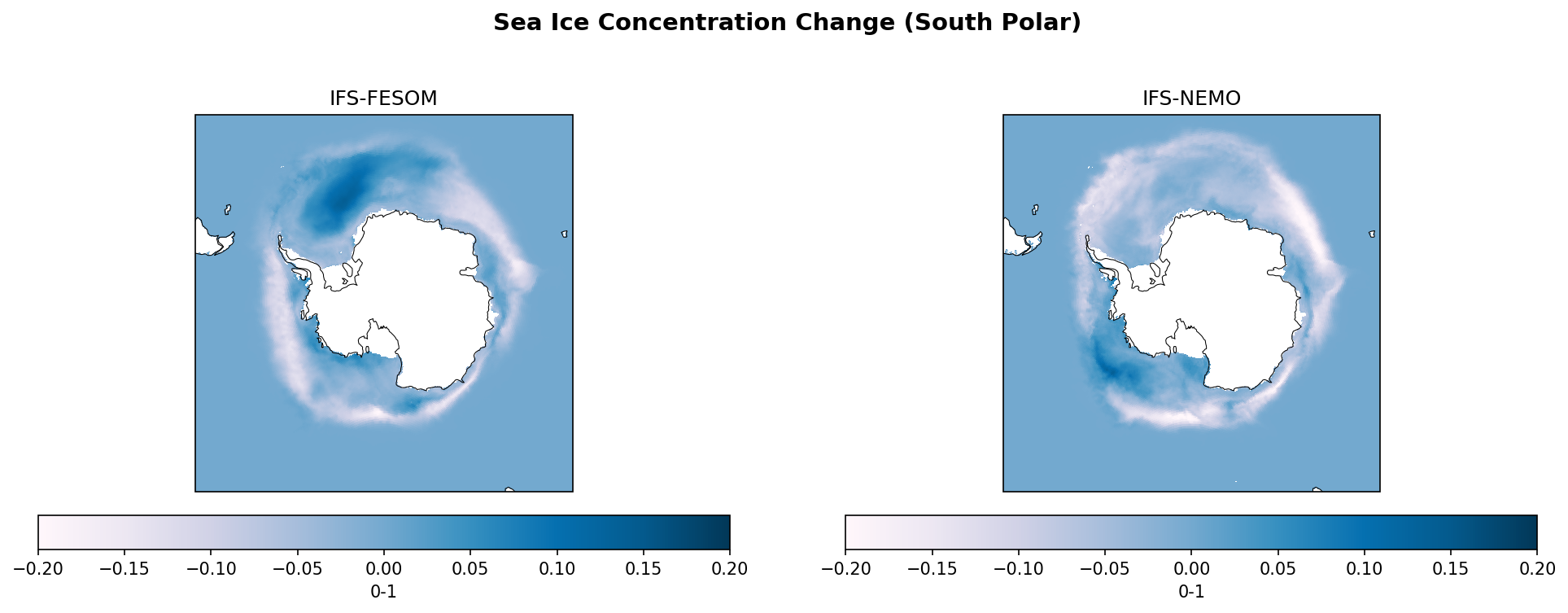
While the CMIP6 multi-model mean projects a widespread circum-Antarctic decline in sea ice concentration by the 2040s, the high-resolution IFS-FESOM and IFS-NEMO models exhibit highly heterogeneous patterns with significant regional sea ice increases that oppose the warming trend.
Key Findings
- CMIP6-MMM shows a robust, nearly annular reduction in sea ice concentration, particularly in the Weddell and Amundsen/Bellingshausen Seas, consistent with thermodynamic warming.
- IFS-FESOM displays a striking dipole pattern: a strong increase in sea ice concentration in the Weddell Sea (contrary to CMIP6), offset by sharp declines in the Amundsen and Bellingshausen sectors.
- IFS-NEMO shows a differing regional anomaly, with sea ice increases concentrated in the Ross Sea sector, while the Weddell Sea and East Antarctic coast experience significant loss.
Spatial Patterns
The CMIP6 response is zonally relatively symmetric and negative (red). IFS-FESOM is dominated by a positive anomaly (blue, >0.15) in the Weddell Gyre region. IFS-NEMO features a positive anomaly in the Ross Sea, with widespread negative anomalies (red) extending from the Weddell Sea eastward around East Antarctica.
Model Agreement
The DestinE models disagree significantly with the CMIP6 mean and with each other regarding regional spatial patterns. While the background signal is likely loss (red), the high-resolution models are dominated by large regional positive anomalies (blue) that are absent in the smoothed multi-model mean.
Physical Interpretation
The strong regional increases in the DestinE models likely reflect internal climate variability (e.g., specific phases of the Southern Annular Mode, Amundsen Sea Low, or Weddell Gyre dynamics) dominating the decadal mean. In single-member simulations over short periods (10 years), dynamic redistribution of ice by wind and currents can locally overwhelm the thermodynamic melting signal that is isolated in the CMIP6 ensemble mean.
Caveats
- The 10-year future averaging period (2040-2049) is short relative to Antarctic variability; results may capture transient decadal noise rather than forced long-term trends.
- Comparisons between single realizations (DestinE) and an ensemble mean (CMIP6) naturally exaggerate differences, as the mean filters out the strong internal variability visible in individual model runs.
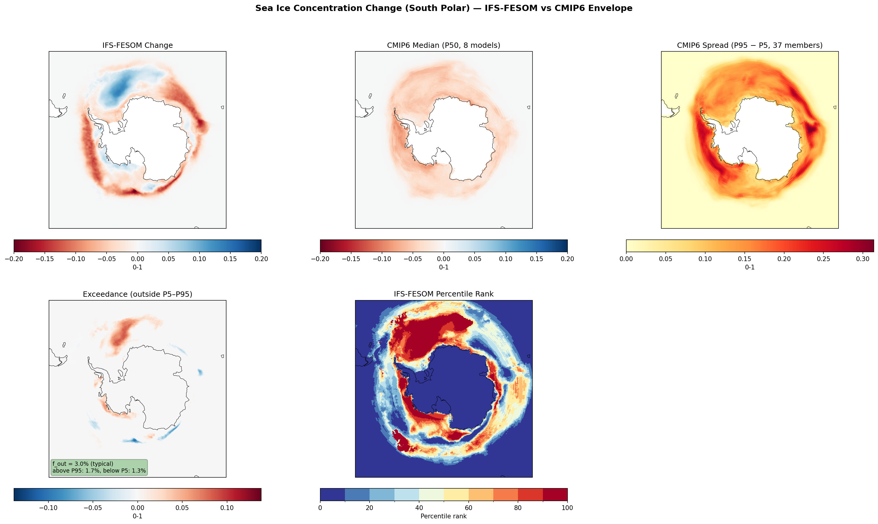
Sea Ice Concentration Change (South Polar) — IFS-FESOM vs CMIP6 Envelope f_out 3.0%
Envelope Metrics
| f_out (outside P5–P95) | 3.0% typical |
|---|---|
| Above P95 | 1.7% |
| Below P5 | 1.3% |
| CMIP6 ensemble | 8 models, 37 members |
| Variables | avg_siconc |
|---|---|
| Models | ifs-fesom |
| Units | 0-1 |
| Baseline | 1990-2014 |
| Future | 2040-2049 |
| Method | Future mean minus historical mean compared to CMIP6 percentile envelope (P5, P50, P95). |
Summary high
IFS-FESOM projects a heterogeneous Southern Ocean sea ice response for the 2040s, featuring expected declines in the Amundsen and Indian sectors but a notable, atypical increase in the Weddell Sea compared to the baseline.
Key Findings
- A distinct region of sea ice concentration increase (blue in Change panel, up to +0.15) is visible in the Weddell Sea, starkly contrasting with the CMIP6 median's uniform decline.
- This Weddell Sea anomaly results in the model exceeding the CMIP6 P95 percentile (red in Exceedance panel), indicating a response at the extreme upper tail of the ensemble distribution.
- Strong sea ice loss occurs in the Amundsen, Bellingshausen, and Indian sectors, where the model frequently falls below the CMIP6 P5 threshold (blue in Exceedance panel), indicating losses stronger than 95% of CMIP6 models.
- Despite these distinct regional anomalies, the global area-weighted f_out is low (3.0%), classifying the deviation as 'typical' overall, largely due to the extremely wide spread of the CMIP6 envelope in the Southern Ocean.
Spatial Patterns
The spatial response is zonally asymmetric. While the CMIP6 median shows a circumpolar ring of sea ice loss, IFS-FESOM shows a dipole: extensive retreat in West Antarctica and the Indian Ocean sector, offset by sea ice expansion/retention in the Weddell Gyre.
Model Agreement
The model generally falls within the CMIP6 envelope (97% of area) because the CMIP6 spread is very high (up to 0.3) along the Antarctic sea ice edge. However, the Percentile Rank panel highlights that IFS-FESOM is often at the extremes (Rank 0 or Rank 100) rather than near the median (Rank 50).
Physical Interpretation
The anomalous sea ice increase in the Weddell Sea is likely driven by internal decadal variability rather than forced climate change. Specifically, this pattern often results from the cessation of deep convection or the closing of a Weddell Polynya (common in high-resolution ocean models) between the baseline and future periods, which would manifest as a local cooling/ice-increase trend masking the global warming signal.
Caveats
- The 10-year averaging period (2040-2049) is short enough that decadal variability (e.g., polynya cycles) can dominate the forced trend.
- The 'increase' in sea ice likely represents a recovery from a low-ice state in the specific baseline realization (1990-2014) rather than a long-term physically forced growth.
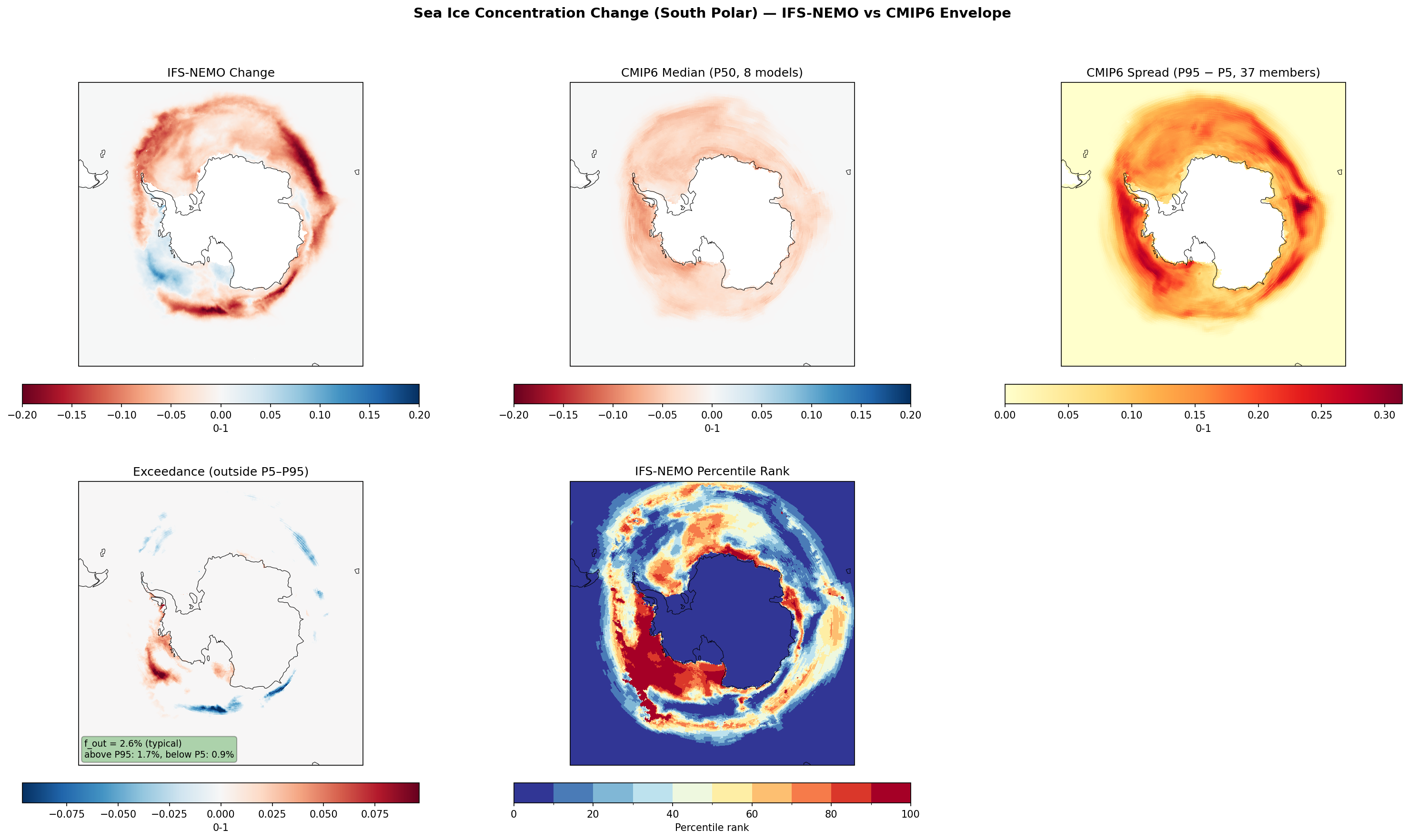
Sea Ice Concentration Change (South Polar) — IFS-NEMO vs CMIP6 Envelope f_out 2.6%
Envelope Metrics
| f_out (outside P5–P95) | 2.6% typical |
|---|---|
| Above P95 | 1.7% |
| Below P5 | 0.9% |
| CMIP6 ensemble | 8 models, 37 members |
| Variables | avg_siconc |
|---|---|
| Models | ifs-nemo |
| Units | 0-1 |
| Baseline | 1990-2014 |
| Future | 2040-2049 |
| Method | Future mean minus historical mean compared to CMIP6 percentile envelope (P5, P50, P95). |
Summary high
IFS-NEMO projects a spatially heterogeneous pattern of Antarctic sea ice change (2040–2049 vs 1990–2014) characterized by a strong dipole of loss in the Weddell Sea and gain in the Amundsen Sea, contrasting with the zonally symmetric loss of the CMIP6 median. Despite these regional structure differences, the model falls largely within the CMIP6 envelope (f_out = 2.6%) due to the significant inter-model spread in Antarctic sea ice projections.
Key Findings
- IFS-NEMO shows a pronounced regional dipole: strong sea ice loss in the Weddell and Ross Seas (anomalies ~ -0.2) contrasting with sea ice concentration increases in the Amundsen and Bellingshausen Seas (anomalies ~ +0.1).
- The CMIP6 median (P50) depicts a smoother, annular pattern of sea ice retreat around the entire continent, notably lacking the sector of sea ice growth seen in the high-resolution model.
- Global agreement is high: only 2.6% of the area lies outside the CMIP6 P5–P95 envelope, confirming that IFS-NEMO's strong regional anomalies are generally within the bounds of CMIP6 structural uncertainty and internal variability.
Spatial Patterns
The dominant feature is the contrast between the Weddell Sea (deep red in change plot, indicating strong decline) and the Amundsen/Bellingshausen sector (blue in change plot, indicating increase). The Exceedance panel highlights that the Weddell Sea loss occasionally exceeds the CMIP6 P95 (red patches), while the Amundsen gain represents a 'negative loss' that falls below the CMIP6 P5 (blue patches).
Model Agreement
IFS-NEMO agrees with the CMIP6 ensemble in predicting general Antarctic sea ice decline but disagrees on the spatial uniformity. The low f_out (2.6%) is driven by the very large spread in CMIP6 projections (Panel 3) in the marginal ice zone, which accommodates the strong dynamic responses seen in IFS-NEMO.
Physical Interpretation
The dipole pattern in IFS-NEMO is characteristic of wind-driven dynamic redistribution, likely associated with the Amundsen Sea Low (ASL). High-resolution models often better resolve the interaction between ASL winds and the Antarctic Peninsula topography, driving meridional ice transport (drift) that creates distinct regions of convergence (thickening/gain) and divergence (loss). The CMIP6 median smooths these dynamic features.
Caveats
- The 10-year future window (2040-2049) is short, meaning internal variability (e.g., ENSO or SAM phasing) likely contributes significantly to the dipole pattern, superimposing on the long-term trend.
- Percentile Rank interpretation: The visual patterns suggest the rank calculation likely treats 'Sea Ice Loss' as a positive quantity (hence regions of gain appear as rank ~0 and strong loss as rank ~100).
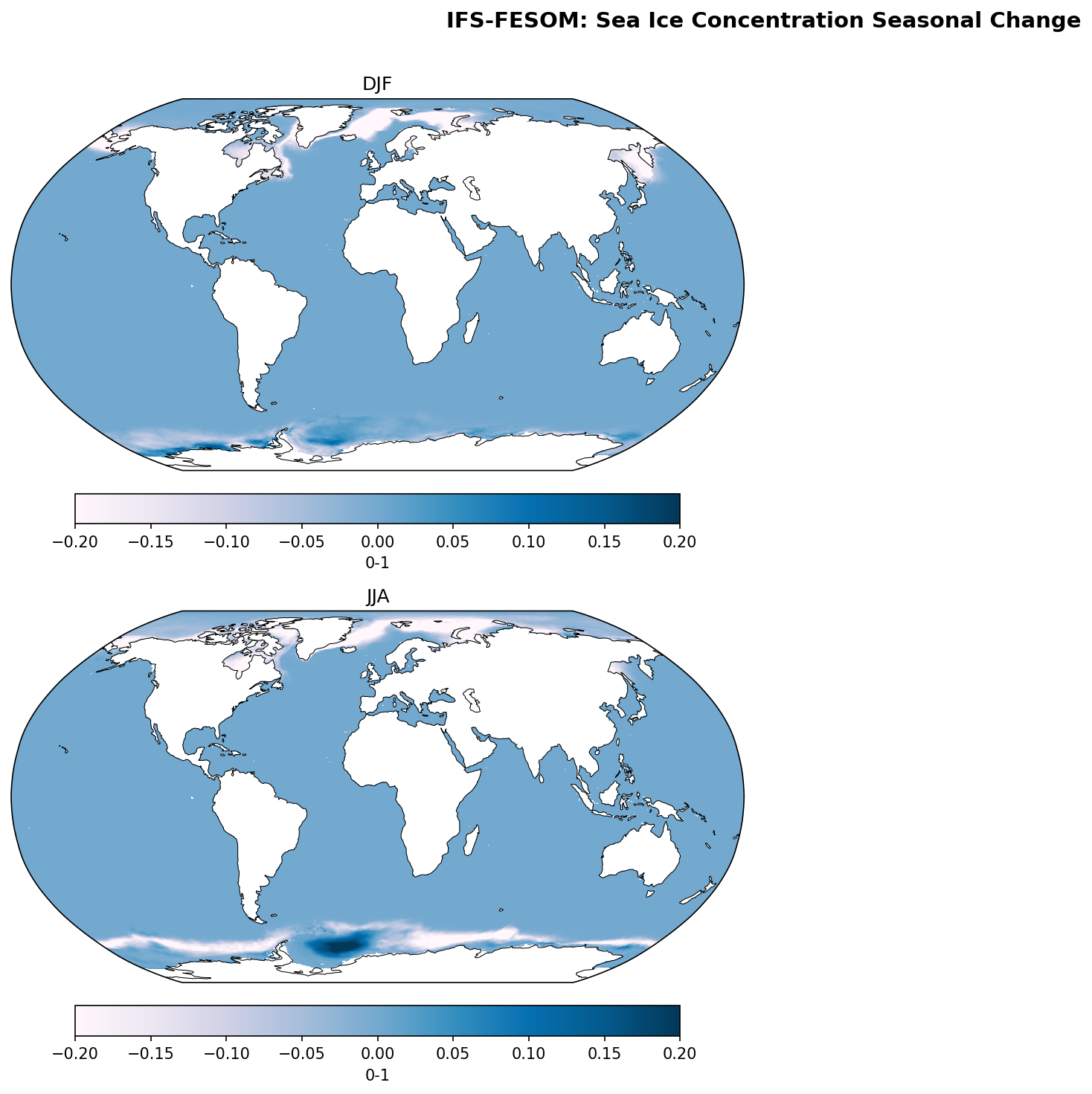
Sea Ice Concentration Seasonal Change — IFS-FESOM
| Variables | avg_siconc |
|---|---|
| Models | ifs-fesom |
| Units | 0-1 |
| Baseline | 1990-2014 |
| Future | 2040-2049 |
| Method | Per-season future mean minus historical mean. |
Summary high
IFS-FESOM projects consistent seasonal sea ice loss across the Arctic marginal zones, while the Antarctic response is highly heterogeneous, featuring a notable region of increased winter sea ice concentration in the Weddell Sea.
Key Findings
- Arctic sea ice concentration decreases significantly in the marginal seas (Barents, Okhotsk, Labrador) during Boreal winter (DJF).
- Arctic Boreal summer (JJA) shows widespread retreat along the Siberian shelf (Laptev, East Siberian seas) and Beaufort Sea.
- Antarctic Austral winter (JJA) exhibits a strong dipole in the Weddell Sea: a distinct region of increased sea ice concentration (>0.15) contrasted with retreat at the ice edge.
- Antarctic Austral summer (DJF) changes are mixed and lower magnitude, with losses concentrated in the Amundsen and Bellingshausen coastal regions.
Spatial Patterns
The Arctic shows a 'rim-like' pattern of loss tracking the seasonal ice edge. The Antarctic displays a complex zonal asymmetry, dominated by the positive anomaly in the Weddell Sea gyre region during JJA, which opposes the general trend of decline at the lower-latitude ice margins.
Model Agreement
The Arctic retreat is consistent with the CMIP6 multi-model mean expectations of thermodynamic sea ice loss (Arctic Amplification). The strong localized increase in the Weddell Sea is likely an outlier compared to the CMIP6 mean, suggesting a model-specific dynamical response (potentially related to resolution) or internal variability phase.
Physical Interpretation
Arctic loss is driven by global warming and the ice-albedo feedback. The counter-intuitive increase in Weddell Sea ice (JJA) likely results from increased upper-ocean stratification (due to freshening/warming) suppressing deep convection or open-ocean polynyas that were present in the baseline simulation. Once convection halts, surface heat flux decreases, allowing ice to reform or thicken.
Caveats
- The 10-year future period (2040-2049) is short relative to Southern Ocean multidecadal variability; the Weddell signal could reflect a phase shift in internal variability rather than a forced trend.
- Comparison of a 25-year baseline to a 10-year future slice may introduce sampling biases.
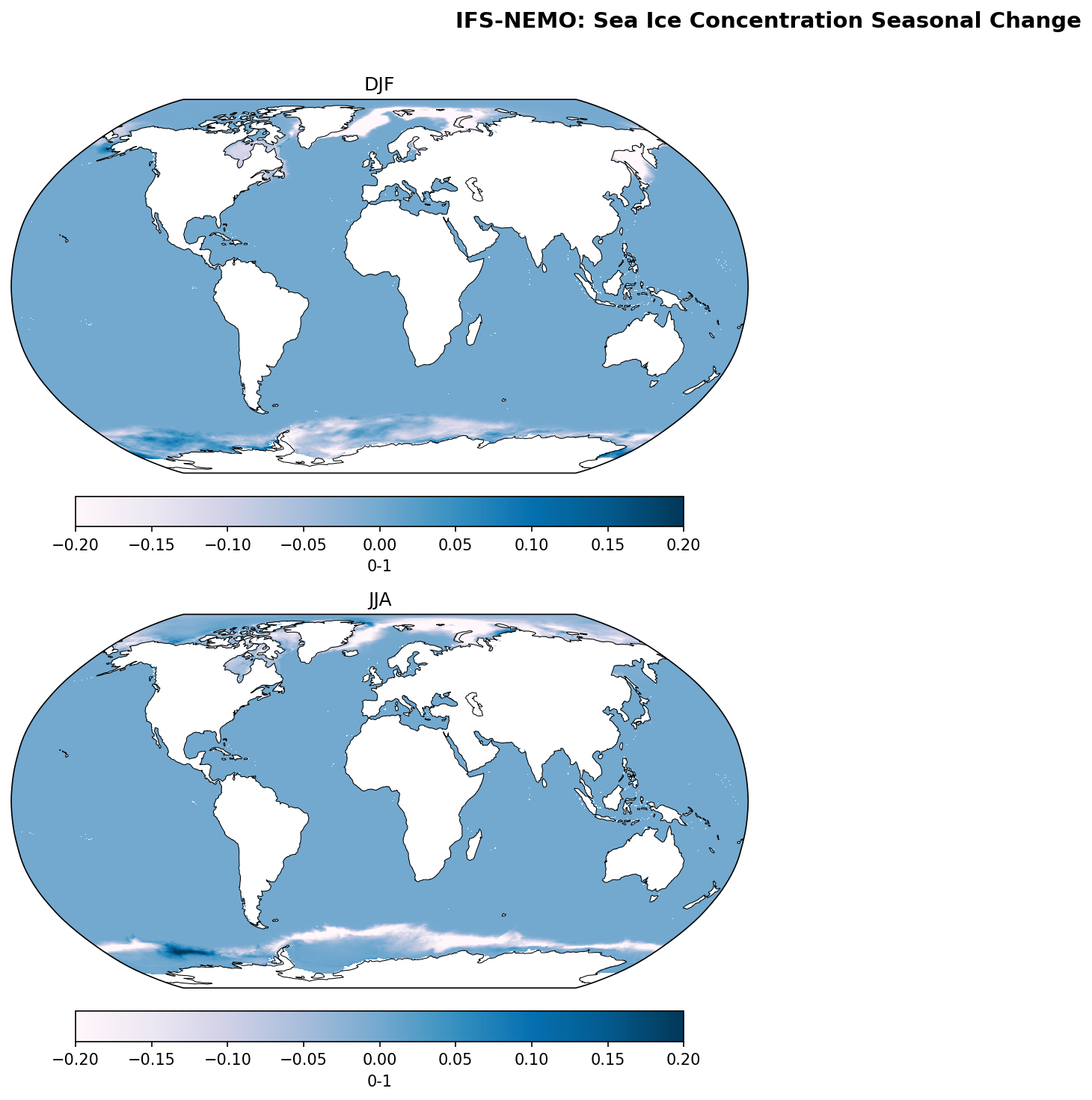
Sea Ice Concentration Seasonal Change — IFS-NEMO
| Variables | avg_siconc |
|---|---|
| Models | ifs-nemo |
| Units | 0-1 |
| Baseline | 1990-2014 |
| Future | 2040-2049 |
| Method | Per-season future mean minus historical mean. |
Summary high
IFS-NEMO projects widespread sea ice concentration decreases by the 2040–2049 period under SSP3-7.0, characterized by seasonal marginal sea ice loss in the Arctic and a circumpolar retreat of the Antarctic winter ice edge.
Key Findings
- Arctic winter (DJF) shows strong sea ice loss focused in the Barents, Kara, and Okhotsk Seas, indicating a retreat of the winter maximum extent.
- Arctic summer (JJA) exhibits broad concentration declines along the Eurasian and North American continental shelves, signaling a reduction in summer sea ice coverage.
- Antarctic winter (JJA) displays a ring of sea ice loss at the northern edge of the pack ice, consistent with thermodynamic warming.
- A localized area of sea ice concentration increase is visible in the Amundsen/Ross Sea sector of the Southern Ocean during JJA.
Spatial Patterns
In the Arctic (DJF), the 'Atlantification' signal is evident with deep reductions (>-0.20) in the Barents Sea. In the Arctic (JJA), loss is circum-Arctic along the coasts. In the Antarctic (JJA), the pattern is largely annular loss at the ice edge (~60°S), disrupted by a dipole pattern in the Pacific sector (strong loss in Bellingshausen vs. slight gain in Amundsen/Ross seas).
Model Agreement
The Arctic patterns, particularly the retreat of sea ice in the Barents and Okhotsk seas, are highly consistent with the broader CMIP6 ensemble response to warming. The Antarctic response is more variable across models; while the general retreat agrees with CMIP6, the specific regional increase in the Amundsen/Ross sector likely reflects IFS-NEMO's specific realization of internal variability (e.g., wind patterns) or structural dynamical response.
Physical Interpretation
Arctic losses are primarily thermodynamic, driven by surface warming and, in the Barents Sea, enhanced ocean heat transport from the Atlantic. The Antarctic pattern suggests a combination of thermodynamic melt (general retreat) and dynamic redistribution; the JJA increase in the Amundsen/Ross sector is likely driven by anomalies in the Amundsen Sea Low causing northward ice advection or convergence.
Caveats
- The analysis compares a short 10-year future period (2040-2049) against the baseline; decadal internal variability could strongly influence regional signals (like the Antarctic dipole).
- No statistical significance masking is applied, so smaller anomalies (especially slight increases) may be within noise levels.
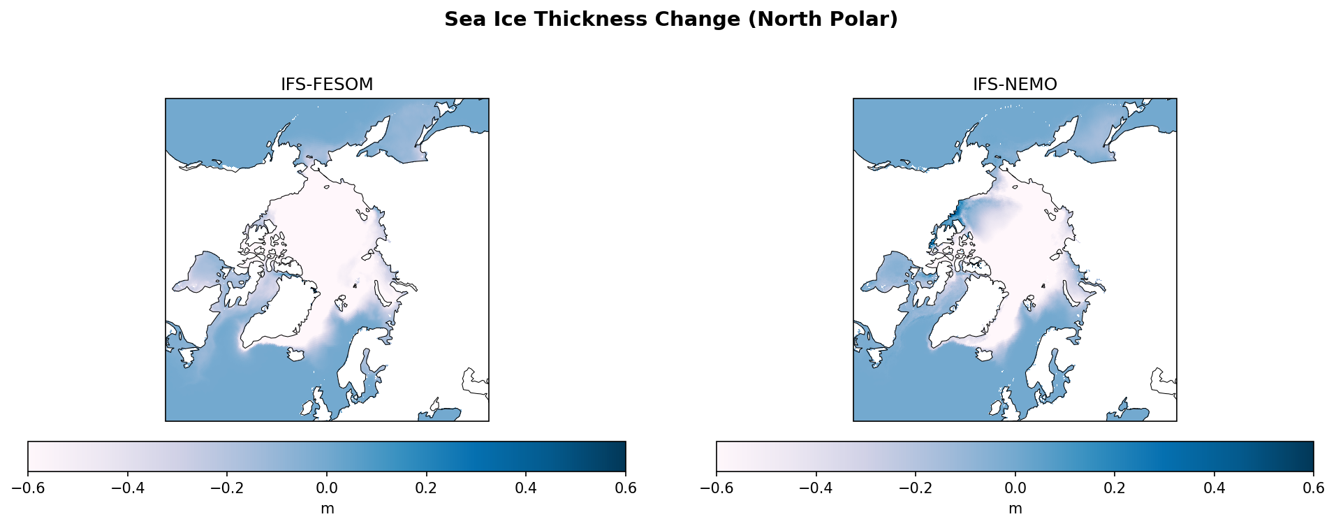
Sea Ice Thickness Change (NH)
| Variables | avg_sithick |
|---|---|
| Models | ifs-fesom, ifs-nemo, CMIP6-MMM |
| Units | m |
| Baseline | 1990-2014 |
| Future | 2040-2049 |
| Method | Future mean minus historical mean. |
Summary high
This figure illustrates the projected annual sea ice thickness change in the North Polar region between the baseline (1990-2014) and the future (2040-2049) under SSP3-7.0. All three panels (IFS-FESOM, IFS-NEMO, and CMIP6-MMM) show a consistent, large-scale reduction in sea ice thickness across the Arctic Basin.
Key Findings
- Widespread sea ice thinning exceeding 0.8 m is observed throughout the central Arctic Ocean in all models.
- IFS-FESOM and CMIP6-MMM show highly similar spatial patterns, with extensive thinning extending into Hudson Bay, Baffin Bay, and the Canadian Archipelago.
- IFS-NEMO predicts intense thinning in the central basin and north of Greenland but shows localized differences in the Canadian Archipelago, where some areas show neutral or slight thickening signals compared to the thinning in FESOM.
Spatial Patterns
The maximum thinning (>0.8 m, dark red) is concentrated in the Central Arctic and the region north of Greenland and the Canadian Archipelago, historically the home of the thickest multi-year ice. Marginal seas (Barents, Kara, Laptev) show moderate thinning, likely bounded by the fact that baseline ice there is already thinner/seasonal.
Model Agreement
There is high agreement between the high-resolution DestinE prototypes and the CMIP6 multi-model mean regarding the sign and general magnitude of sea ice loss. IFS-FESOM appears to track the CMIP6 ensemble mean spatial footprint slightly more closely than IFS-NEMO in the marginal regions (e.g., Hudson Bay).
Physical Interpretation
The patterns reflect the Arctic amplification of global warming, driving thermodynamic melting and the loss of thick multi-year ice via the ice-albedo feedback. The significant thinning in the 'Last Ice Area' (north of Greenland) suggests a potential transition toward a seasonally ice-free Arctic by mid-century.
Caveats
- Change fields are sensitive to baseline mean state; a model with thicker initial ice can exhibit larger absolute thickness reductions.
- The analysis does not distinguish between thermodynamic melt and dynamic export (ice motion) changes.
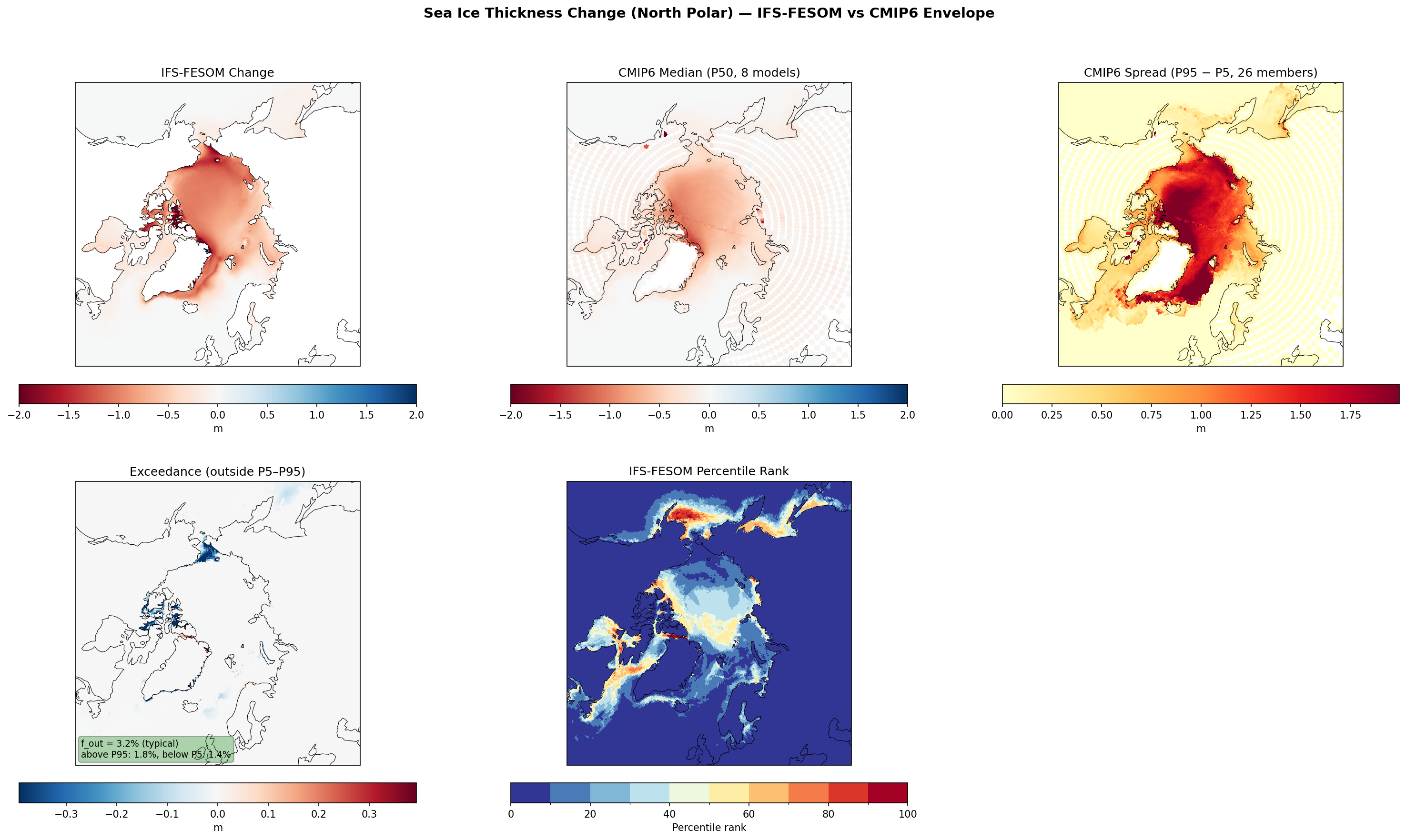
Sea Ice Thickness Change (North Polar) — IFS-FESOM vs CMIP6 Envelope f_out 3.2%
Envelope Metrics
| f_out (outside P5–P95) | 3.2% typical |
|---|---|
| Above P95 | 1.8% |
| Below P5 | 1.4% |
| CMIP6 ensemble | 8 models, 26 members |
| Variables | avg_sithick |
|---|---|
| Models | ifs-fesom |
| Units | m |
| Baseline | 1990-2014 |
| Future | 2040-2049 |
| Method | Future mean minus historical mean compared to CMIP6 percentile envelope (P5, P50, P95). |
Summary high
IFS-FESOM projects extensive Arctic sea ice thinning of 1.0–2.0 m by the 2040s, exhibiting remarkable consistency with the CMIP6 ensemble (f_out = 3.2%) with only minor, localized deviations.
Key Findings
- IFS-FESOM predicts a basin-wide reduction in sea ice thickness, with maxima exceeding 1.5 m loss in the Central Arctic and north of Greenland, closely tracking the CMIP6 median.
- The model behavior is classified as 'typical' (f_out = 3.2%), indicating that the high-resolution simulation lies almost entirely within the uncertainty range of standard-resolution CMIP6 models.
- Regional deviations show IFS-FESOM projecting slightly weaker thinning than the CMIP6 upper bound (P95) in the Lincoln Sea/Canadian Archipelago region, and slightly stronger thinning (below P5) in localized marginal ice zones.
Spatial Patterns
The primary pattern is a strong reduction in thickness across the multi-year ice regions of the Central Arctic. IFS-FESOM shows sharper gradients along the Canadian Archipelago and better resolution of straits compared to the smooth CMIP6 median. The 'Last Ice Area' north of Greenland shows the largest absolute change but also the largest inter-model spread.
Model Agreement
Agreement is very high; the Percentile Rank map is dominated by values between 30 and 70, placing IFS-FESOM near the center of the CMIP6 distribution. The specific disagreement north of Ellesmere Island (Red exceedance) indicates IFS-FESOM retains slightly more thickness there than the bulk of CMIP6 models.
Physical Interpretation
The broad consistency implies that basin-scale thermodynamic melting dominates the signal and is handled similarly in IFS-FESOM as in CMIP6. The deviation in the thickest ice region likely stems from differences in dynamic ice rheology (ridging) or wind-driven export mechanics, which are sensitive to resolution and coastline representation.
Caveats
- The CMIP6 spread (P95-P5) is very large (>1.5 m) in the region north of Greenland, which lowers the bar for 'agreement' (staying within the envelope) in that specific area.
- Analysis is limited to thermodynamic thickness change; extent and concentration changes may show different sensitivities.
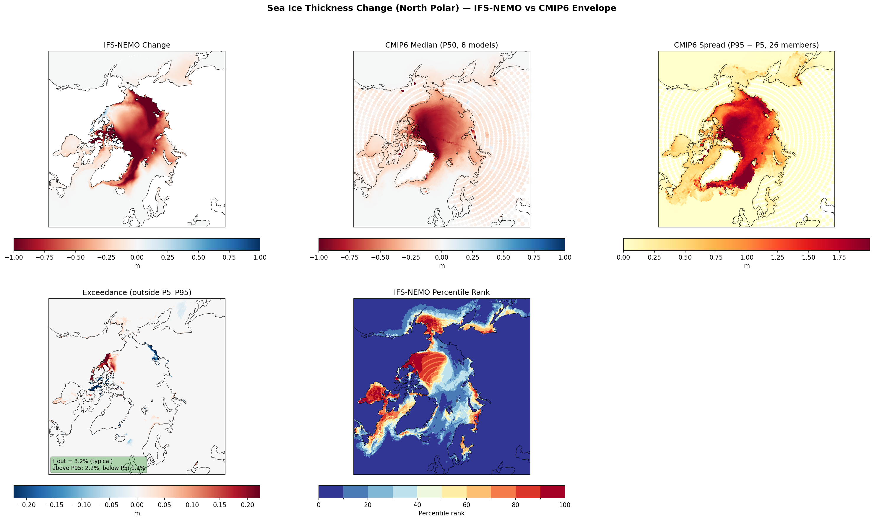
Sea Ice Thickness Change (North Polar) — IFS-NEMO vs CMIP6 Envelope f_out 3.2%
Envelope Metrics
| f_out (outside P5–P95) | 3.2% typical |
|---|---|
| Above P95 | 2.2% |
| Below P5 | 1.1% |
| CMIP6 ensemble | 8 models, 26 members |
| Variables | avg_sithick |
|---|---|
| Models | ifs-nemo |
| Units | m |
| Baseline | 1990-2014 |
| Future | 2040-2049 |
| Method | Future mean minus historical mean compared to CMIP6 percentile envelope (P5, P50, P95). |
Summary high
IFS-NEMO projects widespread Arctic sea ice thinning (-0.5 to -1.5 m) by 2040–2049, exhibiting remarkably high consistency with the CMIP6 ensemble (f_out = 3.2%) while offering improved detail in narrow passageways.
Key Findings
- IFS-NEMO shows robust agreement with the CMIP6 median across the central Arctic basin, with thinning patterns and magnitudes nearly identical to the ensemble average.
- Localized exceedance (stronger thinning than CMIP6 P5) occurs in the Canadian Arctic Archipelago (CAA), likely due to the model's high resolution resolving channels that are closed or unresolved in coarser CMIP6 models.
- The model projects slightly weaker thinning than the CMIP6 median (percentile ranks >70) in the Lincoln Sea and north of Greenland, suggesting greater resilience of the thickest multi-year ice in IFS-NEMO.
Spatial Patterns
The dominant signal is strong negative change (thinning) concentrated north of Greenland and the Canadian Archipelago, coincident with the region of historically thickest ice. The CMIP6 spread is also maximal in this region (>1.5 m), indicating high inter-model uncertainty where ice is thickest.
Model Agreement
Agreement is exceptionally high, with only 3.2% of the area falling outside the CMIP6 P5–P95 envelope. The percentile rank map is dominated by values between 30–70, confirming IFS-NEMO behaves as a 'typical' CMIP6 model for sea ice thickness change.
Physical Interpretation
The broad thinning is thermodynamically driven by Arctic amplification. The specific deviation in the CAA (stronger thinning) reflects added value of high resolution: resolved channels allow for ice export and ocean heat intrusion that coarse models miss. The high agreement elsewhere likely stems from IFS-NEMO sharing the underlying NEMO-SI3/LIM sea ice physics with several contributing CMIP6 models (e.g., EC-Earth3, IPSL-CM6A, CNRM-CM6).
Caveats
- The strong agreement may partly result from model genealogy (shared sea ice components with key CMIP6 members) rather than independent validation.
- Results represent a mid-term (2040s) snapshot; long-term trajectory of the 'Last Ice Area' north of Greenland requires further analysis.
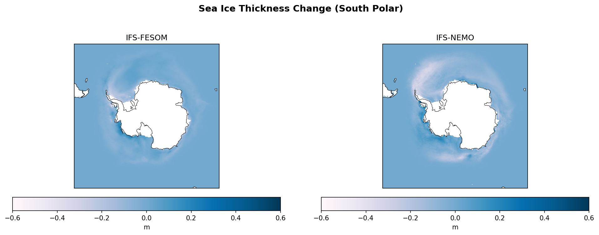
Sea Ice Thickness Change (SH)
| Variables | avg_sithick |
|---|---|
| Models | ifs-fesom, ifs-nemo, CMIP6-MMM |
| Units | m |
| Baseline | 1990-2014 |
| Future | 2040-2049 |
| Method | Future mean minus historical mean. |
Summary medium
This figure compares projected annual Antarctic sea ice thickness changes (2040–2049 relative to 1990–2014) between two high-resolution DestinE models (IFS-FESOM, IFS-NEMO) and the CMIP6 multi-model mean. While all models agree on sea ice loss in the Weddell Sea, they diverge significantly in magnitude and spatial response in the West Antarctic sector.
Key Findings
- IFS-NEMO projects the most severe and widespread sea ice loss, with thinning exceeding 0.4–0.6 m across most sectors, particularly the Weddell and Ross Seas.
- IFS-FESOM predicts more moderate thinning (-0.2 m range) and exhibits distinct localized coastal thickening features not seen in the other panels.
- The CMIP6-MMM displays a zonal asymmetry: thinning in the Weddell/East Antarctic sectors contrasted by notable thickening (up to +0.4 m) in the Amundsen and Bellingshausen Seas, a feature absent in the IFS models.
Spatial Patterns
The Weddell Sea is a region of consistent thinning across all models, though magnitudes vary. The most striking spatial discrepancy is in the Amundsen/Bellingshausen sector (West of the Peninsula), where CMIP6 shows thickening (blue), IFS-FESOM shows weak signals, and IFS-NEMO shows strong thinning (red). IFS-FESOM uniquely resolves narrow bands of thickening pressed against the coastline, likely representing dynamic ridging or coastal convergence.
Model Agreement
Models agree on the sign of change (loss) in the Weddell Sea and Indian Ocean sector. Disagreement is high in the Pacific sector (West Antarctica), where CMIP6 suggests potential thickening versus strong loss in IFS-NEMO. IFS-NEMO is the outlier for total volume loss, appearing much more sensitive to warming than the ensemble mean.
Physical Interpretation
The widespread thinning in IFS-NEMO may indicate a strong thermodynamic response or issues with Southern Ocean deep convection (common in some NEMO configurations) leading to enhanced basal melt. The CMIP6 thickening pattern likely reflects dynamic redistribution driven by changes in the Amundsen Sea Low, which the high-resolution IFS runs may simulate differently or override with stronger thermodynamic melting. The coastal thickening in IFS-FESOM demonstrates the added value of unstructured grids in resolving coastline-ice interactions.
Caveats
- Antarctic sea ice trends are subject to high internal variability; a 10-year future window may capture decadal phasing rather than just the forced trend.
- The CMIP6 mean smoothes over individual model biases, whereas the single realizations of IFS-NEMO/FESOM expose specific model internal variability (e.g., potential open-ocean polynyas).
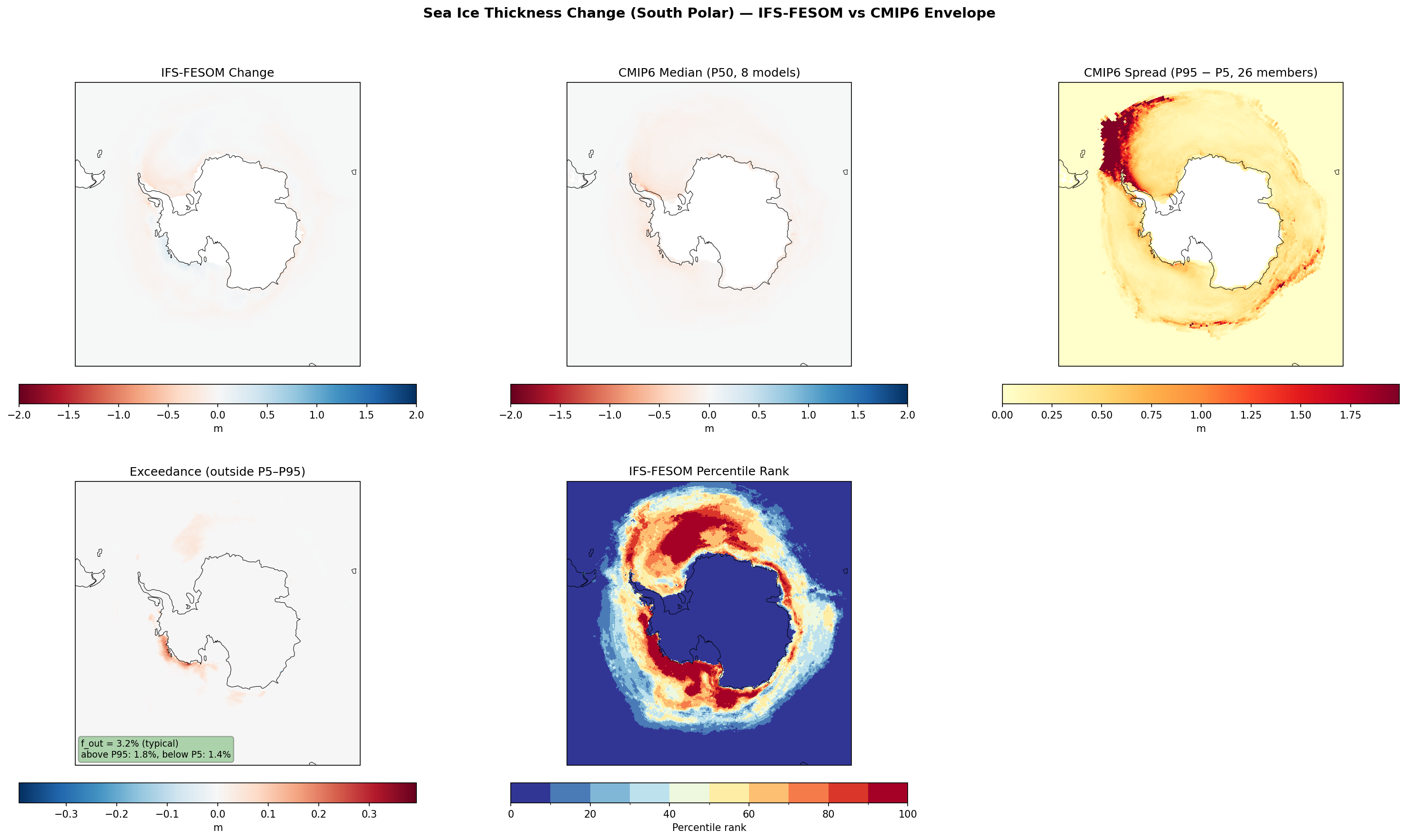
Sea Ice Thickness Change (South Polar) — IFS-FESOM vs CMIP6 Envelope f_out 3.2%
Envelope Metrics
| f_out (outside P5–P95) | 3.2% typical |
|---|---|
| Above P95 | 1.8% |
| Below P5 | 1.4% |
| CMIP6 ensemble | 8 models, 26 members |
| Variables | avg_sithick |
|---|---|
| Models | ifs-fesom |
| Units | m |
| Baseline | 1990-2014 |
| Future | 2040-2049 |
| Method | Future mean minus historical mean compared to CMIP6 percentile envelope (P5, P50, P95). |
Summary high
IFS-FESOM projects widespread Antarctic sea ice thinning (0.5–1.5 m) by the 2040s, showing exceptional agreement with the CMIP6 ensemble distribution. With only 3.2% of the area falling outside the CMIP6 P5–P95 envelope, the model's response is statistically typical, falling well within the substantial uncertainty spread of the coarser models.
Key Findings
- IFS-FESOM projects dominant sea ice thinning in the Weddell, Ross, and Amundsen Seas, with magnitudes generally between -0.5 m and -1.5 m.
- The model shows high consistency with CMIP6; `f_out` is 3.2% (typical), indicating almost no significant outliers relative to the ensemble spread.
- Percentile analysis reveals IFS-FESOM sits at the upper end of the distribution (less thinning than median) in the Weddell Sea, but at the lower end (stronger thinning than median) in the Amundsen/Bellingshausen sector.
Spatial Patterns
The dominant feature is thinning in the perennial ice zones of the Weddell and Ross Seas. The CMIP6 spread is largest in the Weddell Sea (>1.5 m), reflecting high model uncertainty in this region. IFS-FESOM exhibits a dipole in relative behavior: it is 'less aggressive' than the CMIP6 median in the Weddell Sea (high percentile ranks) but 'more aggressive' in the Amundsen Sea (low percentile ranks).
Model Agreement
Agreement is very high. The `f_out` metric (3.2%) is well below the threshold for atypical behavior. The Exceedance panel is largely empty, confirming IFS-FESOM's changes are almost entirely subsumed by the (admittedly wide) CMIP6 envelope.
Physical Interpretation
The patterns reflect thermodynamic sea ice loss under SSP3-7.0 warming. The large CMIP6 spread in the Weddell Sea likely relates to variability in deep convection and polynya formation processes among models; IFS-FESOM's high percentile rank there suggests it maintains stratification or ice volume better than the most sensitive CMIP6 members. Conversely, dynamic losses or ocean heat flux in the Amundsen sector may be more pronounced in the high-resolution eddy-permitting FESOM ocean compared to the CMIP6 median.
Caveats
- The CMIP6 spread (P95-P5) is extremely large in the Weddell Sea (up to 1.75 m), making it easier for the model to fall within the envelope.
- Results depend on baseline ice thickness; if IFS-FESOM starts with thicker/thinner ice than CMIP6, potential change is constrained differently.
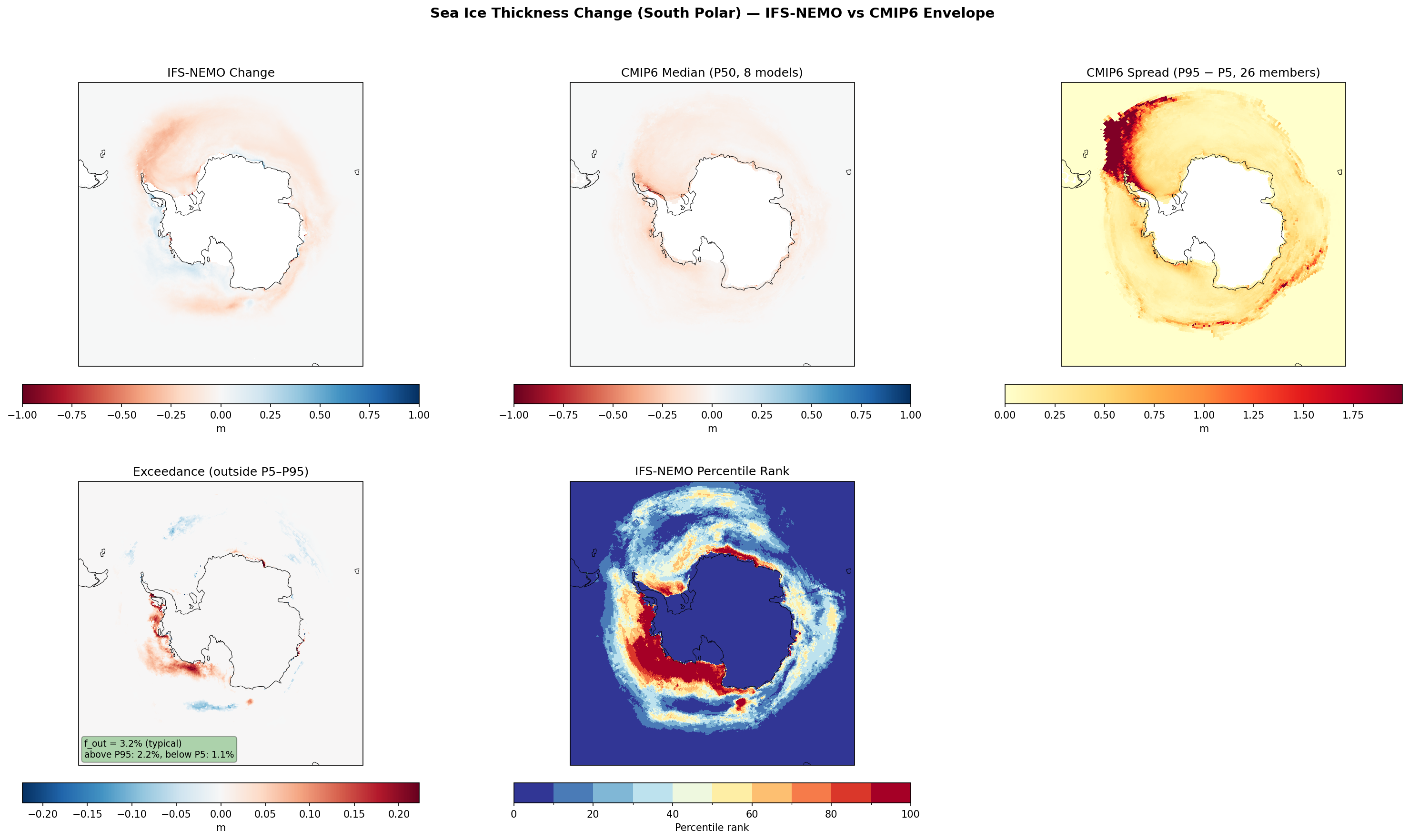
Sea Ice Thickness Change (South Polar) — IFS-NEMO vs CMIP6 Envelope f_out 3.2%
Envelope Metrics
| f_out (outside P5–P95) | 3.2% typical |
|---|---|
| Above P95 | 2.2% |
| Below P5 | 1.1% |
| CMIP6 ensemble | 8 models, 26 members |
| Variables | avg_sithick |
|---|---|
| Models | ifs-nemo |
| Units | m |
| Baseline | 1990-2014 |
| Future | 2040-2049 |
| Method | Future mean minus historical mean compared to CMIP6 percentile envelope (P5, P50, P95). |
Summary high
IFS-NEMO projects widespread Antarctic sea ice thinning (up to 0.75 m) by 2040–2049, generally tracking the CMIP6 median pattern with high consistency (f_out = 3.2%). While the model falls well within the broad CMIP6 envelope, it exhibits a distinct spatial structure with stronger thinning at the ice edge and relative ice retention (or thickening) in the coastal Weddell Sea compared to the ensemble.
Key Findings
- IFS-NEMO is highly consistent with the CMIP6 ensemble (f_out 3.2%, labeled 'typical'), indicating no widespread outlier behaviour.
- The CMIP6 spread in the Weddell Sea is extremely large (>1.5 m), indicating high uncertainty in standard models which IFS-NEMO falls within.
- IFS-NEMO shows a distinct 'dipole' of behavior in the Weddell Sea: stronger thinning than average at the outer ice edge (low percentile rank), but weaker thinning or thickening near the Antarctic Peninsula (high percentile rank, >90).
Spatial Patterns
The dominant pattern is sea ice thinning around the Antarctic continent, particularly in the Weddell and Ross Seas. A notable feature is the western Weddell Sea along the Antarctic Peninsula, where IFS-NEMO predicts less thinning (or slight thickening) compared to the CMIP6 median, indicated by red regions in the Exceedance panel and high percentile ranks. Conversely, the marginal ice zones often show lower percentile ranks (blue), suggesting sharper or stronger retreat/thinning at the ice edge in IFS-NEMO.
Model Agreement
IFS-NEMO agrees well with the CMIP6 ensemble on the sign and general magnitude of change. The very low f_out (3.2%) suggests it is a representative realization within the uncertainty bounds. The large CMIP6 spread (yellow/red in top-right panel) implies a weak constraint, making it easier for the high-resolution model to stay within the envelope.
Physical Interpretation
The preservation of thicker ice in the western Weddell Sea (high percentile rank) likely reflects the added value of high resolution in resolving the Weddell Gyre circulation and ice rheology. High-resolution models can better simulate the mechanical pile-up of sea ice against the Antarctic Peninsula (convergence) compared to coarser CMIP6 models, which may smear this dynamic feature. The stronger thinning at the drift edge may reflect more active ocean eddies bringing heat to the surface or a sharper frontal definition.
Caveats
- The large spread in the CMIP6 envelope (>1.5m in key regions) means that 'agreement' is partly due to the high uncertainty of the baseline ensemble rather than precise alignment.
- Antarctic sea ice trends are dominated by high internal variability; the 2040-2049 window may capture specific phases of variability (e.g., polynyas) differently than the ensemble mean.
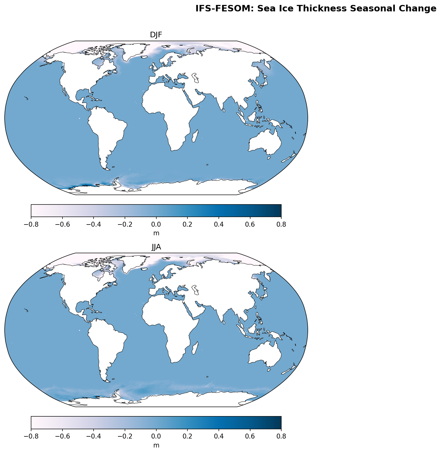
Sea Ice Thickness Seasonal Change — IFS-FESOM
| Variables | avg_sithick |
|---|---|
| Models | ifs-fesom |
| Units | m |
| Baseline | 1990-2014 |
| Future | 2040-2049 |
| Method | Per-season future mean minus historical mean. |
Summary high
IFS-FESOM projects widespread and severe sea ice thinning across the Arctic in both winter and summer by the 2040s, contrasted with a spatially heterogeneous response in the Antarctic featuring a dipole of thinning and localized thickening.
Key Findings
- The Arctic Ocean exhibits extensive sea ice thinning exceeding 0.8 m (saturation of the color scale) in both DJF and JJA, particularly north of Greenland and the Canadian Archipelago.
- Antarctic sea ice change is regionally asymmetric; in Austral winter (JJA), there is notable thickening in the Amundsen/Ross Sea sectors contrasting with thinning in the Weddell Sea and East Antarctic coast.
- Arctic thinning is persistent across seasons, indicating a decline in multi-year ice volume, whereas Antarctic changes show stronger seasonality aligned with the expansion of the seasonal ice zone.
Spatial Patterns
In the Northern Hemisphere, the strongest negative anomalies target the 'Last Ice Area' north of the Canadian Archipelago and Greenland, as well as the central Arctic basin. In the Southern Hemisphere, a dipole pattern is evident in JJA: thinning (red) in the Weddell Sea and thickening (blue) in the Amundsen/Bellingshausen/Ross Sea sector. Small patches of thickening also appear near the Antarctic coast in DJF.
Model Agreement
The strong Arctic decline is consistent with the broad CMIP6 consensus under SSP3-7.0 (Arctic Amplification). The complex Antarctic dipole pattern—showing regions of growth amidst general warming—is often associated with internal variability (e.g., phasing of the Amundsen Sea Low) or specific coupled model dynamics, which varies significantly across the CMIP6 ensemble.
Physical Interpretation
Arctic loss is driven by thermodynamic warming and the ice-albedo feedback, leading to the rapid depletion of thick multi-year ice. The Antarctic pattern suggests dynamic drivers, where changes in atmospheric circulation (winds) drive ice advection, causing convergence (thickening) in the Amundsen/Ross sector and divergence/export (thinning) elsewhere.
Caveats
- The 10-year future window (2040-2049) is relatively short, meaning the specific Antarctic spatial pattern may be heavily influenced by internal decadal variability rather than a forced long-term trend.
- The color scale saturates at ±0.8 m, likely masking the full magnitude of loss in the thickest Arctic ice regions.
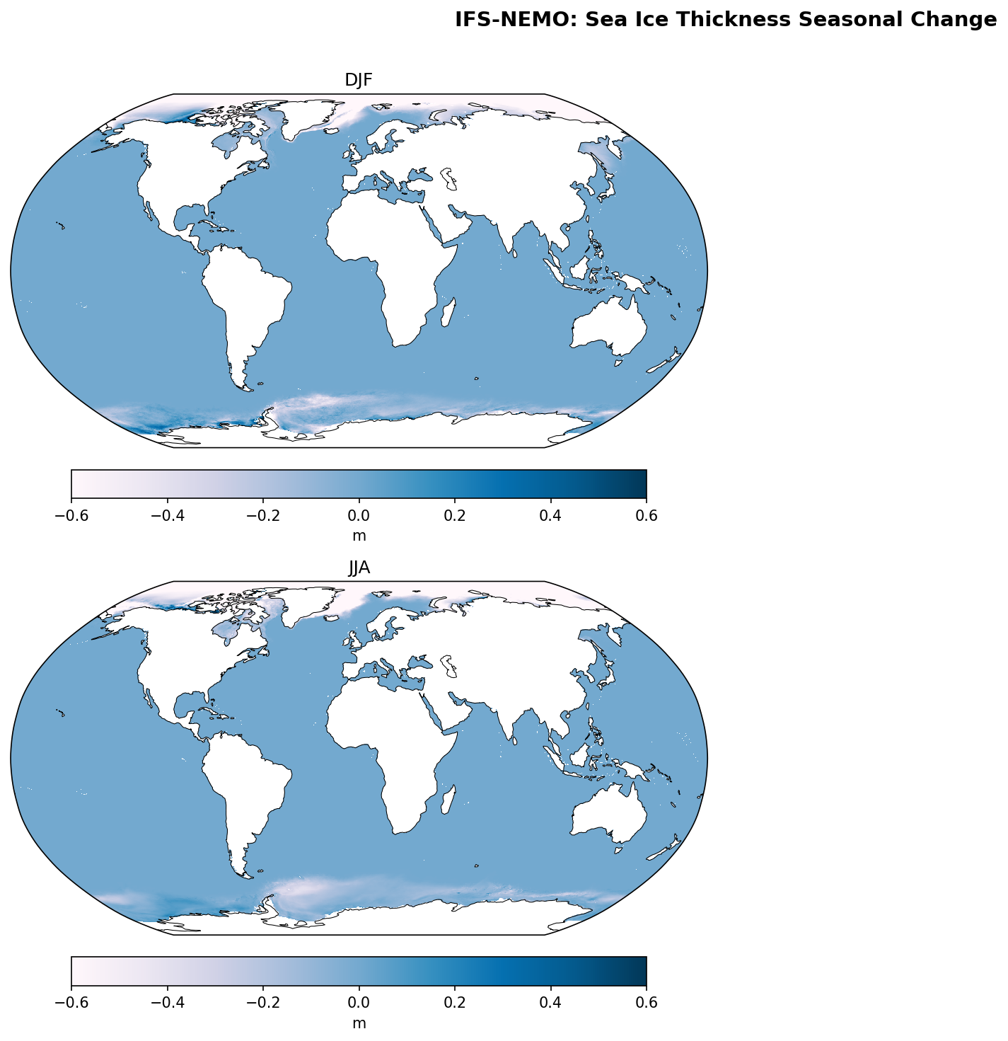
Sea Ice Thickness Seasonal Change — IFS-NEMO
| Variables | avg_sithick |
|---|---|
| Models | ifs-nemo |
| Units | m |
| Baseline | 1990-2014 |
| Future | 2040-2049 |
| Method | Per-season future mean minus historical mean. |
Summary high
IFS-NEMO projects extensive sea ice thinning across both poles by 2040–2049 relative to the 1990–2014 baseline under SSP3-7.0, with Arctic losses exceeding 0.6 m in the central basin and Antarctic losses concentrated in the Weddell Sea.
Key Findings
- Arctic sea ice thickness decreases by over 0.6 m across the Central Arctic and north of Greenland (the 'Last Ice Area') in both seasons, indicating a severe reduction in multi-year ice volume.
- The Weddell Sea in the Antarctic exhibits the strongest regional thinning signal (<-0.6 m) in both seasons, suggesting a weakening of the perennial ice pack or enhanced ocean heat flux in this sector.
- Seasonal differences are marked in the Arctic marginal seas, with significant thinning in the Barents and Kara seas in DJF (winter) that is less prominent in JJA (summer), likely due to the seasonal ice edge retreat.
Spatial Patterns
Arctic thinning is widespread but most intense north of the Canadian Archipelago, coincident with the climatological location of the thickest multi-year ice. Antarctic changes are highly asymmetrical; the Weddell and Ross Seas show deep thinning, whereas the Amundsen/Bellingshausen sectors show weak thinning or localized thickening (DJF).
Model Agreement
Comparison panels are not provided, but the magnitude of central Arctic thinning aligns with the high-sensitivity subset of CMIP6 models under SSP3-7.0. The pronounced Weddell Sea thinning is a feature often sensitive to ocean model resolution and vertical mixing (open-ocean convection) in NEMO configurations, which may differ from the coarser CMIP6 multi-model mean.
Physical Interpretation
Arctic decline is driven by Arctic Amplification and the ice-albedo feedback, leading to the preferential melt of thick multi-year ice. The strong Weddell Sea thinning suggests a dynamic or thermodynamic change in the Weddell Gyre, possibly linked to warm deep water intrusion or convective mixing inhibiting winter ice growth.
Caveats
- Without a pre-industrial control run, it is difficult to fully distinguish the forced climate change signal from potential model drift, particularly in the sensitive Antarctic region.
- The projection window is near-term (2040s), meaning internal climate variability could still play a significant role in regional patterns (e.g., Southern Ocean modes).
Sea Ice Volume per Area Change (NOH)
| Variables | avg_sivol |
|---|---|
| Models | ifs-fesom, ifs-nemo |
| Units | m |
| Baseline | 1990-2014 |
| Future | 2040-2049 |
| Method | Future mean minus historical mean. |
Summary high
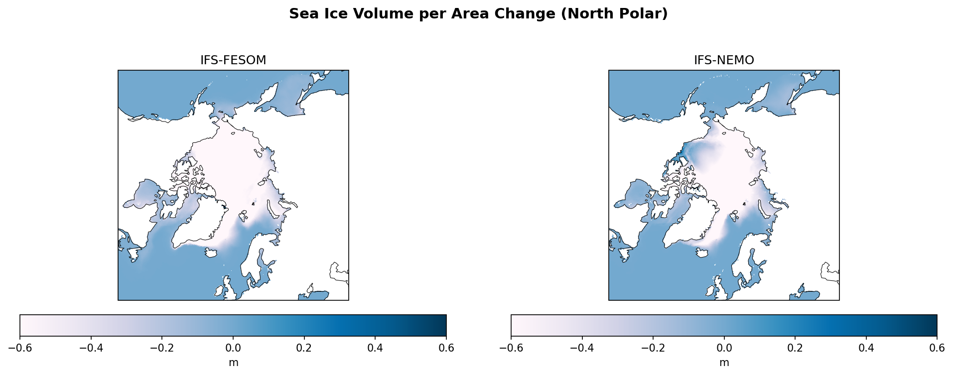
Both IFS-FESOM and IFS-NEMO project extensive reductions in Arctic sea ice volume per area (effective thickness) by 2040–2049 relative to the 1990–2014 baseline, with widespread declines exceeding 0.6 m across the central Arctic basin.
Key Findings
- The central Arctic experiences severe sea ice thinning, with losses saturating the color scale (>0.6 m) in both models.
- The strongest volume reductions align with historical regions of thick multi-year ice (north of Greenland and the Canadian Archipelago), indicating a potential regime shift to thinner first-year ice.
- IFS-FESOM projects more extensive thinning in marginal seas (e.g., Sea of Okhotsk, Hudson Bay) compared to IFS-NEMO, suggesting different baseline ice extents or sensitivities in these regions.
- IFS-NEMO exhibits a localized area of stability or slight thickening in the Beaufort Sea, contrasting with the strong thinning seen there in IFS-FESOM.
Spatial Patterns
Both models show a dominant 'red' signal of volume loss across the entire Arctic Ocean, particularly along the Transpolar Drift stream and north of the Canadian Archipelago. A notable divergence occurs in the Beaufort Gyre region (north of Alaska), where IFS-FESOM shows deep thinning (dark red), while IFS-NEMO shows a patch of neutral to slight positive change (light blue/white). IFS-FESOM also shows clearer thinning signals in the Sea of Okhotsk and Labrador Sea compared to IFS-NEMO.
Model Agreement
There is strong agreement on the sign and magnitude of sea ice loss in the central Arctic and the East Greenland export route. Disagreement is primarily dynamic: the handling of the Beaufort Gyre leads to different thickness responses (likely convergence in NEMO vs. thinning in FESOM), and the marginal ice zone extent differs in the peripheral seas.
Physical Interpretation
The pervasive thinning is driven by Arctic amplification (thermodynamic melt) and the reduction of multi-year ice volume, which historically survived summer melt. The losses north of Greenland suggest increased export through the Fram Strait or in-situ melting of the oldest ice. The discrepancy in the Beaufort Sea likely arises from differences in wind-driven ice convergence (rheology) and ocean surface circulation between the unstructured grid (FESOM) and structured grid (NEMO) formulations.
Caveats
- The color scale saturates at ±0.6 m, likely masking the true magnitude of thinning in the central Arctic, where multi-year ice loss can exceed several meters.
- The analysis relies on a single realization per model, so internal variability cannot be fully disentangled from structural model differences.
Sea Ice Volume per Area Change (SOH)

| Variables | avg_sivol |
|---|---|
| Models | ifs-fesom, ifs-nemo |
| Units | m |
| Baseline | 1990-2014 |
| Future | 2040-2049 |
| Method | Future mean minus historical mean. |
Summary high
IFS-NEMO projects widespread and substantial sea ice volume loss in the Southern Ocean, particularly in the Weddell Sea, whereas IFS-FESOM shows a much weaker, heterogeneous signal with localized regions of volume increase.
Key Findings
- IFS-NEMO exhibits strong sea ice volume reduction (reaching -0.6 m) across the Weddell Sea and East Antarctic sectors, indicating significant thinning.
- IFS-FESOM displays a muted response with generally weak magnitude changes (within ±0.2 m) and unexpected areas of ice volume gain (blue) in the inner Weddell Sea and off East Antarctica.
- There is a fundamental disagreement in sensitivity: IFS-NEMO suggests rapid degradation of the Antarctic cryosphere by the 2040s, while IFS-FESOM suggests resistance or dynamic redistribution.
Spatial Patterns
IFS-NEMO features a coherent, high-magnitude arc of volume loss dominating the Weddell Sea and extending eastward into the Indian Ocean sector. In contrast, IFS-FESOM shows scattered, slight thinning near the Antarctic Peninsula and Ross Sea, interspersed with diffuse patches of thickening in the Weddell Gyre and along the East Antarctic coast.
Model Agreement
Low agreement. The models disagree on the sign of change in the Weddell Gyre and East Antarctic sectors and differ significantly on the magnitude of loss in the marginal ice zones.
Physical Interpretation
The widespread volume loss in IFS-NEMO is consistent with thermodynamic melting driven by oceanic and atmospheric warming under SSP3-7.0. The anomalous thickening or lack of loss in IFS-FESOM implies different sea ice rheology/dynamics (convergence) or distinct ocean states; specifically, if IFS-FESOM simulated deep convection/polynyas in the baseline but not the future, volume could appear to increase. The unstructured grid of FESOM may also resolve shelf processes and water mass formation differently, affecting heat flux to the ice.
Caveats
- The short 10-year averaging period (2040-2049) makes the analysis susceptible to multi-decadal internal variability (e.g., variations in the Weddell Gyre strength or SAM), which can mask the forced trend.
- Without baseline thickness maps, it is unclear if IFS-FESOM's weak change is due to having very little thick ice to lose initially, or robust ice that resists melting.
Sea Ice Volume per Area Seasonal Change — IFS-FESOM
| Variables | avg_sivol |
|---|---|
| Models | ifs-fesom |
| Units | m |
| Baseline | 1990-2014 |
| Future | 2040-2049 |
| Method | Per-season future mean minus historical mean. |
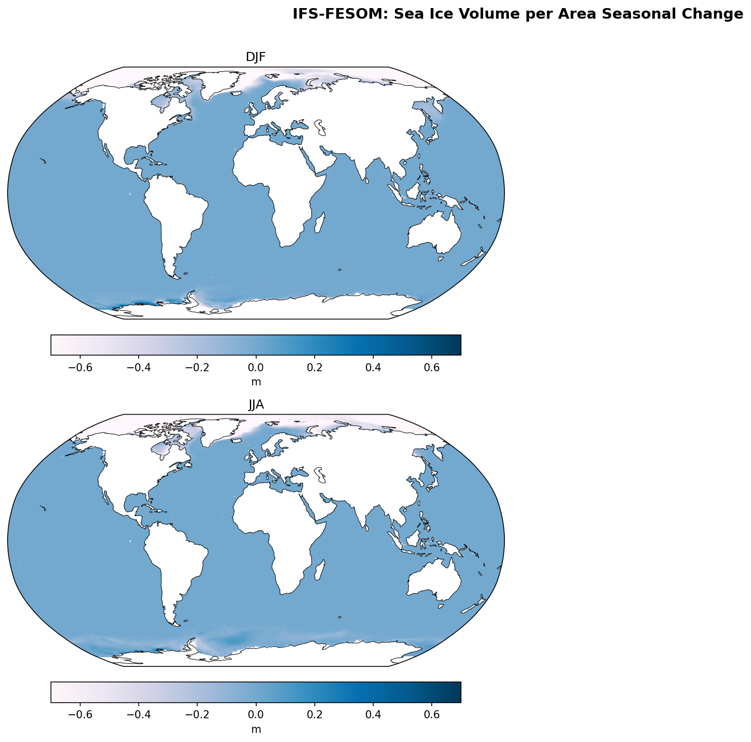
Summary high
IFS-FESOM projects widespread and intense sea ice thinning in the Arctic (>0.6 m loss) across both seasons by the 2040s, whereas the Antarctic exhibits a spatially heterogeneous response with regional thickening in the Ross/Amundsen sector during austral winter.
Key Findings
- The Arctic experiences severe sea ice volume reduction in both DJF and JJA, with losses exceeding 0.6 m (saturated scale) throughout the Central Arctic and the region north of Greenland/Canada.
- Antarctic sea ice changes are zonally asymmetric, particularly in JJA (austral winter), featuring a dipole pattern of thickening in the Ross/Amundsen sector and thinning in the Weddell and Indian Ocean sectors.
- The magnitude of projected Arctic volume loss is significantly larger and more uniform than the mixed signals observed in the Southern Ocean.
Spatial Patterns
In the Arctic, the strongest thinning is concentrated in the multi-year ice regions north of the Canadian Archipelago and Greenland. In the Antarctic during JJA, a notable region of ice volume increase (blue, ~0.2–0.4 m) is visible in the Pacific sector, contrasting with widespread marginal thinning elsewhere.
Model Agreement
The drastic reduction in Arctic sea ice volume is consistent with the broad CMIP6 consensus for SSP3-7.0. The Antarctic dipole pattern (regional thickening) is less robust across models and likely reflects internal variability or specific circulation responses (e.g., Amundsen Sea Low dynamics) captured at this resolution.
Physical Interpretation
Arctic loss is driven by strong thermodynamic warming and the ice-albedo feedback, depleting the reservoir of thick multi-year ice. The Antarctic pattern suggests dynamic redistribution driven by wind stress changes (potentially linked to SAM or ASL variability) rather than uniform thermodynamic melt.
Caveats
- The future averaging period (2040–2049) is only 10 years, meaning internal decadal variability likely heavily influences the Antarctic spatial pattern.
- No statistical significance masking is applied, so smaller signals in the Antarctic may not be robust.
Sea Ice Volume per Area Seasonal Change — IFS-NEMO
| Variables | avg_sivol |
|---|---|
| Models | ifs-nemo |
| Units | m |
| Baseline | 1990-2014 |
| Future | 2040-2049 |
| Method | Per-season future mean minus historical mean. |
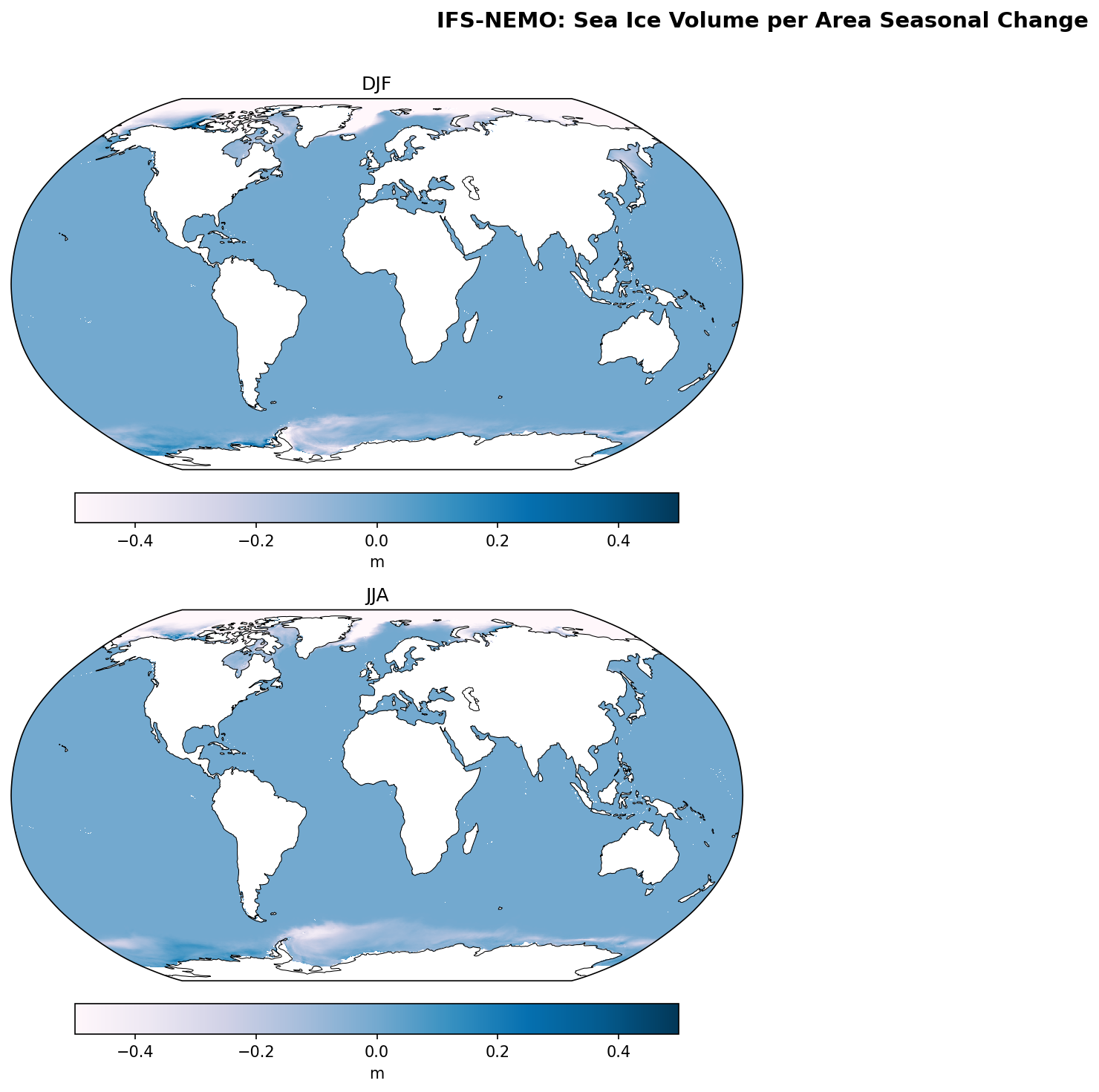
Summary high
IFS-NEMO projects widespread and substantial thinning of Arctic sea ice in both winter and summer by 2040–2049, while Antarctic responses are regionally heterogeneous, dominated by loss in the Weddell Sea.
Key Findings
- Arctic sea ice volume per area shows a robust, basin-wide decrease (>0.4 m) in both DJF and JJA, particularly in the Central Arctic and North of Greenland.
- The Antarctic region exhibits a complex spatial pattern: significant thinning is evident in the Weddell Sea sector in both seasons, whereas the Amundsen and Ross Sea sectors show mixed signals with localized areas of thickening (blue) in austral summer (DJF).
- Seasonal consistency is high in the Arctic (loss in both seasons), suggesting a decline in multi-year ice volume.
- Antarctic changes are generally lower in magnitude and less spatially coherent than those in the Arctic.
Spatial Patterns
The Arctic displays a coherent pattern of loss concentrated in the central basin and the Canadian Archipelago (the traditional 'Last Ice Area'). The Antarctic displays a dipole-like zonal asymmetry, with pronounced volume loss in the Weddell Gyre region and slight gains or neutral conditions in parts of the West Antarctic sector (Amundsen/Bellingshausen) during DJF.
Model Agreement
Although explicit CMIP6 panels are absent, the strong Arctic thinning is qualitatively consistent with the multi-model consensus for SSP3-7.0. The heterogeneous Antarctic signal aligns with the high inter-model spread and internal variability known to characterize Southern Ocean projections in current generation climate models.
Physical Interpretation
Arctic losses are driven by strong polar amplification and the thermodynamic imbalance melting thick multi-year ice. The complex Antarctic pattern likely arises from the interplay of atmospheric circulation changes (e.g., trends in the Southern Annular Mode) and ocean dynamics, where wind-driven redistribution can locally increase ice volume despite global warming.
Caveats
- The future integration period (2040–2049) is short, so internal decadal variability may superimpose onto the forced climate signal, particularly in the highly variable Southern Ocean.
- Volume per area is a combined metric of thickness and concentration; distinct changes in concentration vs. thickness cannot be separated in this view.